Modeling

Guidelines and Rubric

hurricane <- DAAG::hurricNamed
select <- dplyr::select
hurricane <- hurricane %>% select(-c("BaseDamage", "firstLF", 
    "AffectedStates", "LF.times")) %>% na.omit()
hurricane <- hurricane %>% mutate(Category = cut(LF.WindsMPH, 
    breaks = c(-Inf, 74, 95, 110, 129, 156, Inf), labels = c("Trop_Storm", 
        "One", "Two", "Three", "Four", "Five")))

The dataset I have chosen is from the DAAG package, and it is called hurricNamed. This dataset consists of 94 observations of 11 different variables about the named hurricanes that actually made it to the US from the years of 1950 to 2012. The variables I will be using for this project are the gender of the name, the maximum sustained windspeed, the atmospheric pressure at landfall, the property damage in millions of US dollars (adjusted to 2014 inflation level for consistency), the damage that accured (had the hurricane hit the US in 2014), and the number of ensuing deaths. From the details provided by the authors of this data, these data were the subject of a paper that asserted that female-named hurricanes caused more damage than male-named hurricanes due to people taking the female-named hurricanes with less seriousness. This is quite the assertion, and I would like to find if this is actually correct. Immediately off the bat, I converted the windspeed data into the actual categories of the hurricanes with wind measurements provided by the NOAA National Hurricane Center. This not only provides a categorical variable to work with in this project, but it also puts the hurricanes’ power into perspective (people are more familiar with categories than with raw windspeeds).

• 1. MANOVA testing

man1 <- manova(cbind(deaths, LF.PressureMB, NDAM2014, BaseDam2014) ~ 
    Category, data = hurricane)
summary(man1)

## Df Pillai approx F num Df den Df Pr(>F)
## Category 4 1.1017 8.4578 16 356 < 2.2e-16 ***
## Residuals 89
## ---
## Signif. codes: 0 '***' 0.001 '**' 0.01 '*' 0.05 '.' 0.1
' ' 1

summary.aov(man1)

## Response deaths :
## Df Sum Sq Mean Sq F value Pr(>F)
## Category 4 119607 29902 0.7753 0.5441
## Residuals 89 3432446 38567
##
## Response LF.PressureMB :
## Df Sum Sq Mean Sq F value Pr(>F)
## Category 4 26670 6667.5 61.878 < 2.2e-16 ***
## Residuals 89 9590 107.8
## ---
## Signif. codes: 0 '***' 0.001 '**' 0.01 '*' 0.05 '.' 0.1
' ' 1
##
## Response NDAM2014 :
## Df Sum Sq Mean Sq F value Pr(>F)
## Category 4 6.5131e+09 1628283466 9.457 2.038e-06 ***
## Residuals 89 1.5324e+10 172177856
## ---
## Signif. codes: 0 '***' 0.001 '**' 0.01 '*' 0.05 '.' 0.1
' ' 1
##
## Response BaseDam2014 :
## Df Sum Sq Mean Sq F value Pr(>F)
## Category 4 1.4109e+09 352717324 2.3404 0.0611 .
## Residuals 89 1.3413e+10 150708791
## ---
## Signif. codes: 0 '***' 0.001 '**' 0.01 '*' 0.05 '.' 0.1
' ' 1

pairwise.t.test(hurricane$deaths, hurricane$Category, p.adj = "none")

## 
##  Pairwise comparisons using t tests with pooled SD 
## 
## data:  hurricane$deaths and hurricane$Category 
## 
##       One  Two  Three Four
## Two   0.99 -    -     -   
## Three 0.18 0.26 -     -   
## Four  0.43 0.46 0.99  -   
## Five  0.32 0.33 0.60  0.62
## 
## P value adjustment method: none

pairwise.t.test(hurricane$LF.PressureMB, hurricane$Category, 
    p.adj = "none")

## 
##  Pairwise comparisons using t tests with pooled SD 
## 
## data:  hurricane$LF.PressureMB and hurricane$Category 
## 
##       One     Two     Three   Four  
## Two   3.1e-07 -       -       -     
## Three < 2e-16 7.2e-07 -       -     
## Four  3.1e-16 6.7e-08 0.0173  -     
## Five  9.0e-14 3.4e-09 2.0e-05 0.0056
## 
## P value adjustment method: none

pairwise.t.test(hurricane$NDAM2014, hurricane$Category, p.adj = "none")

## 
##  Pairwise comparisons using t tests with pooled SD 
## 
## data:  hurricane$NDAM2014 and hurricane$Category 
## 
##       One     Two     Three   Four   
## Two   0.55811 -       -       -      
## Three 0.02178 0.15321 -       -      
## Four  0.00026 0.00189 0.02208 -      
## Five  3.7e-06 1.3e-05 9.3e-05 0.01386
## 
## P value adjustment method: none

pairwise.t.test(hurricane$BaseDam2014, hurricane$Category, p.adj = "none")

## 
##  Pairwise comparisons using t tests with pooled SD 
## 
## data:  hurricane$BaseDam2014 and hurricane$Category 
## 
##       One   Two   Three Four 
## Two   0.813 -     -     -    
## Three 0.080 0.200 -     -    
## Four  0.498 0.626 0.701 -    
## Five  0.010 0.015 0.049 0.046
## 
## P value adjustment method: none

# Checking probability of Type 1 Error
1 - (0.95^4)

## [1] 0.1854938

0.05/21

## [1] 0.002380952

pairwise.t.test(hurricane$deaths, hurricane$Category, p.adj = "bonf")

## 
##  Pairwise comparisons using t tests with pooled SD 
## 
## data:  hurricane$deaths and hurricane$Category 
## 
##       One Two Three Four
## Two   1   -   -     -   
## Three 1   1   -     -   
## Four  1   1   1     -   
## Five  1   1   1     1   
## 
## P value adjustment method: bonferroni

pairwise.t.test(hurricane$LF.PressureMB, hurricane$Category, 
    p.adj = "bonf")

## 
##  Pairwise comparisons using t tests with pooled SD 
## 
## data:  hurricane$LF.PressureMB and hurricane$Category 
## 
##       One     Two     Three  Four  
## Two   3.1e-06 -       -      -     
## Three < 2e-16 7.2e-06 -      -     
## Four  3.1e-15 6.7e-07 0.1727 -     
## Five  9.0e-13 3.4e-08 0.0002 0.0558
## 
## P value adjustment method: bonferroni

pairwise.t.test(hurricane$NDAM2014, hurricane$Category, p.adj = "bonf")

## 
##  Pairwise comparisons using t tests with pooled SD 
## 
## data:  hurricane$NDAM2014 and hurricane$Category 
## 
##       One     Two     Three   Four   
## Two   1.00000 -       -       -      
## Three 0.21784 1.00000 -       -      
## Four  0.00257 0.01892 0.22077 -      
## Five  3.7e-05 0.00013 0.00093 0.13858
## 
## P value adjustment method: bonferroni

pairwise.t.test(hurricane$BaseDam2014, hurricane$Category, p.adj = "bonf")

## 
##  Pairwise comparisons using t tests with pooled SD 
## 
## data:  hurricane$BaseDam2014 and hurricane$Category 
## 
##       One  Two  Three Four
## Two   1.00 -    -     -   
## Three 0.80 1.00 -     -   
## Four  1.00 1.00 1.00  -   
## Five  0.10 0.15 0.49  0.46
## 
## P value adjustment method: bonferroni

Overall, I am running tests with 4 different numeric variables (deaths,LF.PressureMB,NDAM2014, and BaseDam2014) against the categorical variable I have chosen, which is the category of the hurricanes. From the results of the MANOVA, there are significant differences between hurricane categories for all 5 different variables (Pillai=1.1346, pseudo f-val(20,352)= 6.969, p-val=2.481e-16). From the summary.aov of the MANOVA, it appears that the landfall pressure readings, the number of landfalls, and the damage each hurricane did (if it had appeared in 2014) all significantly differ by category type (LF.Pressure: F-Val=61.878,p-val=2.2e-16; NDAM2014: F-val=9.457,p-val=2.038e-06). I have done 21 hypothesis tests total (1 MANOVA, 4 ANOVA, 16T). The probability of having made a type 1 error is ~18.5% which is quite high. That means that the Bonferroni Adjustment to assure the type 1 error rate stays at 0.05 is 0.05/21, which is 0.002380952. After the Bonferroni adjustment, it does not appear that the significance of these elements changes to become unsignificant.

• 2. Randomization test

hurricane %>% group_by(mf) %>% summarize(m = mean(LF.WindsMPH)) %>% 
    summarize(diff(m))

## # A tibble: 1 x 1
##   `diff(m)`
##       <dbl>
## 1     -3.20

hurricane$mf %>% as.factor()

## [1] f m m f f f f f f f m f f f f f f f f f f f f f f f
f f f f f f f f f f f f f m m m m f f m m f
## [49] f m f f m m f f m m m m f f f f f m f m m m m f f f
f m m m f m f f m f f f f m f m m f m f
## Levels: f m

rand_dist <- vector()
for (i in 1:5000) {
    new <- data.frame(windspeed = sample(hurricane$LF.WindsMPH), 
        mf = hurricane$mf)
    rand_dist[i] <- mean(new[new$mf == "m", ]$windspeed) - mean(new[new$mf == 
        "f", ]$windspeed)
}

mean(rand_dist < -3.203125) * 2  #pvalue

## [1] 0.5252

t.test(data = hurricane, LF.WindsMPH ~ mf)

##
## Welch Two Sample t-test
##
## data: LF.WindsMPH by mf
## t = 0.61536, df = 51.292, p-value = 0.541
## alternative hypothesis: true difference in means is not
equal to 0
## 95 percent confidence interval:
## -7.24555 13.65180
## sample estimates:
## mean in group f mean in group m
## 105.7031 102.5000

{
    hist(rand_dist, main = "", ylab = "")
    abline(v = -3.203125, col = "red")
}

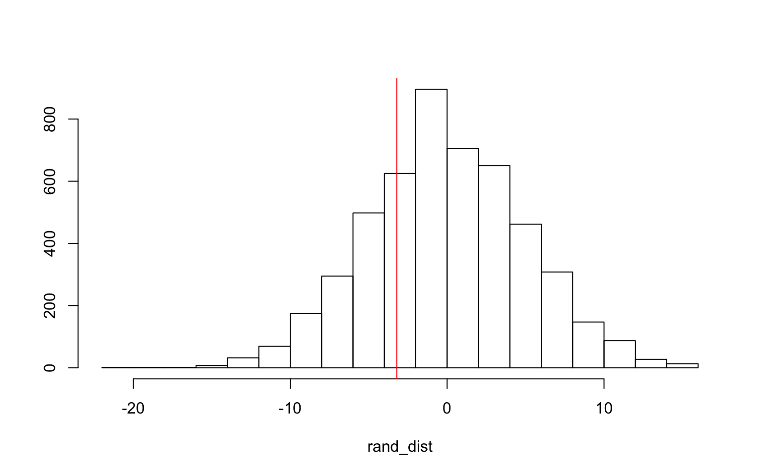Here, the permutation test I used is the Monte Carlo permutation on the standard deviations of the windspeed data from this dataset. Here, the null hypothesis is that the mean windspeed is the same for female named hurricanes and male named hurricanes. The alternative hypothesis is that the mean windspeeds are different between male and female named hurricanes. The p-value received from this test is 0.5012, which means that the null hypothesis is not rejeced, and it looks like there isn’t a difference in windspeeds between male and female named hurricanes (which is a logical conclusion).

• 3. Building a linear regression model predicting one of the response variables from at least 2 other variables, including their interaction.

hurricane$damage_c <- hurricane$BaseDam2014 - mean(hurricane$BaseDam2014)
hurricane$wind_c <- hurricane$LF.WindsMPH - mean(hurricane$LF.WindsMPH)
hurricane$pressure_c <- hurricane$LF.PressureMB - mean(hurricane$LF.PressureMB)

fit1 <- lm(deaths ~ damage_c * pressure_c, data = hurricane)
summary(fit1)

##
## Call:
## lm(formula = deaths ~ damage_c * pressure_c, data =
hurricane)
##
## Residuals:
## Min 1Q Median 3Q Max
## -560.52 -19.98 -6.36 7.21 407.26
##
## Coefficients:
## Estimate Std. Error t value Pr(>|t|)
## (Intercept) -1.183e+01 1.161e+01 -1.019 0.3109
## damage_c -5.189e-03 2.369e-03 -2.190 0.0311 *
## pressure_c -1.801e+00 6.243e-01 -2.885 0.0049 **
## damage_c:pressure_c -4.750e-04 5.825e-05 -8.154 1.96e-12
***
## ---
## Signif. codes: 0 '***' 0.001 '**' 0.01 '*' 0.05 '.' 0.1
' ' 1
##
## Residual standard error: 90.78 on 90 degrees of freedom
## Multiple R-squared: 0.7912, Adjusted R-squared: 0.7842
## F-statistic: 113.7 on 3 and 90 DF, p-value: < 2.2e-16

From this linear regression, there were some very interesting results from predicting the number of deaths from damages done and landfall atmospheric pressures of the hurricanes in this dataset. While controlling for landfall atmospheric pressure, the damages done explain a significant amount of the variation in resulting deaths. For every one point increase in damages, there is a -5.189e-03 increase in resulting deaths. While controlling for damages done, the landfall atmospheric pressures of each hurricane do explain a significant amount of the variation in resulting deaths. Here, for every one unit increase in pressure, there is a -1.801 decrease in death rates. This is due to the fact that lower atmospheric pressures make hurricanes more powerful (or any storm for that matter), so as pressure increases, there are lower deaths. And finally, for the interaction, the effect of damage on death rates is not the same across the different levels of atmospheric pressure (t-val=-8.154, p-val=1.96e-12). For every unit increase in damages across levels of atmospheric pressure, there is a corresponding decrease of -4.750e-04 in resulting deaths.

interact_plot(fit1, damage_c, pressure_c)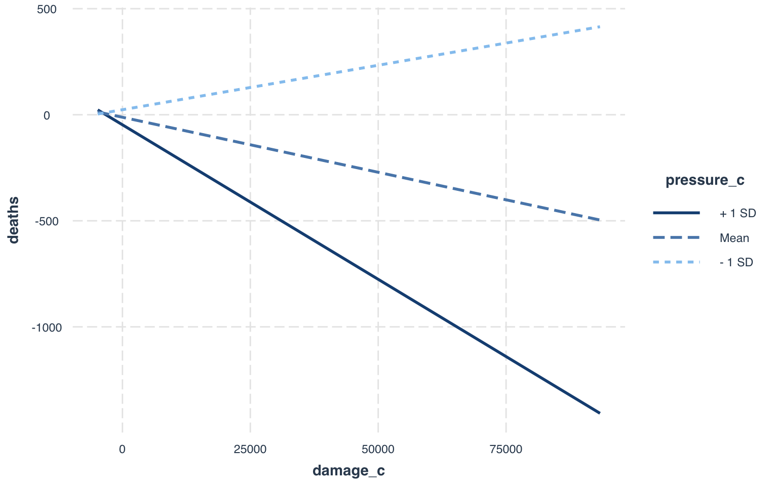

resids <- fit1$residuals
fitvals <- fit1$fitted.values
ggplot() + geom_point(aes(fitvals, resids)) + geom_hline(yintercept = 0, 
    col = "red")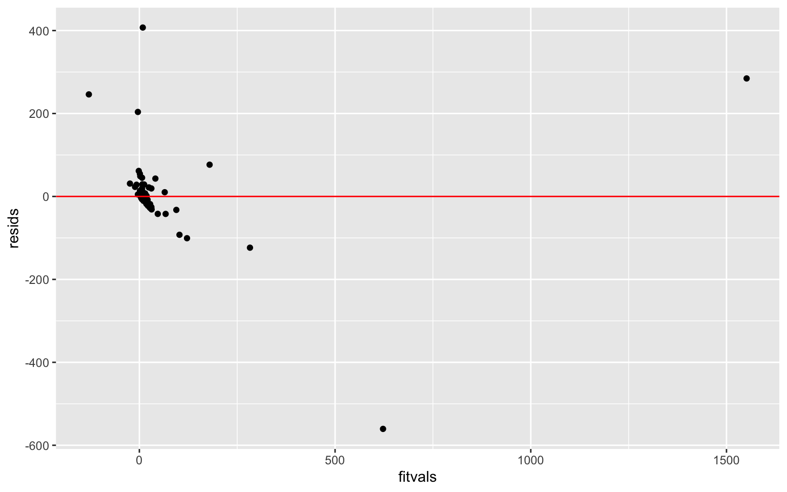

ggplot() + geom_histogram(aes(resids), bins = 20)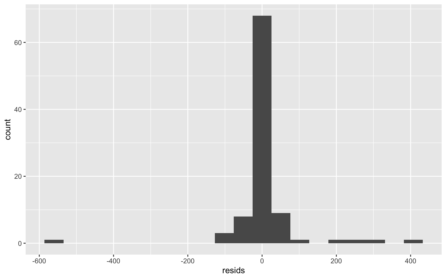

ggplot() + geom_qq(aes(sample = resids)) + geom_qq_line(aes(sample = resids), 
    color = "red")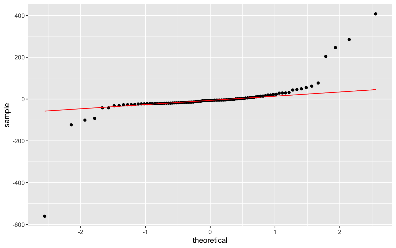

This data does not seem to exhibit homoskedasticity or normality. However, linearity seems to be upheld.

shapiro.test(resids)

## 
##  Shapiro-Wilk normality test
## 
## data:  resids
## W = 0.54612, p-value = 1.424e-15

Shapiro-Wilk’s test has a signifiant p-value, so it means that the normality assumption is violated and the data are not normaly distributed.

bptest(fit1)

## 
##  studentized Breusch-Pagan test
## 
## data:  fit1
## BP = 22.449, df = 3, p-value = 5.259e-05

The Breusch-Pagan test gave a p-value of 5.259e-05 which is significant. This means that the null hypothesis of homoskedasticity is rejected and heteroskedasticity is assumed. The regression should be redone using heteroskedasticity robust SEs to adjust for heteroskedasticity and to be able to use this linear regression model.

coeftest(fit1)[, 1:2]

##                          Estimate   Std. Error
## (Intercept)         -1.183273e+01 1.161213e+01
## damage_c            -5.188969e-03 2.369308e-03
## pressure_c          -1.800907e+00 6.242604e-01
## damage_c:pressure_c -4.749976e-04 5.825146e-05

coeftest(fit1, vcov = vcovHC(fit1))[, 1:2]

##                          Estimate   Std. Error
## (Intercept)         -1.183273e+01 4.372953e+01
## damage_c            -5.188969e-03 8.445183e-03
## pressure_c          -1.800907e+00 1.577618e+00
## damage_c:pressure_c -4.749976e-04 5.122976e-04

From the normal-theory SEs from this linear regression, the significant effects on deaths are damages and the interaction of damages and pressure. After recomputing the regression results with robust standard errors, there were no changes in significance of the variables used. The only notable change was the interaction becoming a little bit less significant.

(sum((deaths - mean(deaths))^2) - sum(fit1$residuals^2))/sum((deaths - 
    mean(deaths))^2)

## [1] 0.9719109

The proportion of the variation in the outcome that the model explains is 0.9719109. The R-squared value from the fit1 regression is 0.7912 (adjusted R-squared = 0.7842).

• 4. Rerunning the same regression model (with interaction), but this time, bootstrapped standard errors are computed.

fit1 <- lm(deaths ~ damage_c * pressure_c, data = hurricane)
summary(fit1)

##
## Call:
## lm(formula = deaths ~ damage_c * pressure_c, data =
hurricane)
##
## Residuals:
## Min 1Q Median 3Q Max
## -560.52 -19.98 -6.36 7.21 407.26
##
## Coefficients:
## Estimate Std. Error t value Pr(>|t|)
## (Intercept) -1.183e+01 1.161e+01 -1.019 0.3109
## damage_c -5.189e-03 2.369e-03 -2.190 0.0311 *
## pressure_c -1.801e+00 6.243e-01 -2.885 0.0049 **
## damage_c:pressure_c -4.750e-04 5.825e-05 -8.154 1.96e-12
***
## ---
## Signif. codes: 0 '***' 0.001 '**' 0.01 '*' 0.05 '.' 0.1
' ' 1
##
## Residual standard error: 90.78 on 90 degrees of freedom
## Multiple R-squared: 0.7912, Adjusted R-squared: 0.7842
## F-statistic: 113.7 on 3 and 90 DF, p-value: < 2.2e-16

samp_distn <- replicate(5000, {
    boot_dat <- boot_dat <- hurricane[sample(nrow(hurricane), 
        replace = TRUE), ]
    fit <- lm(deaths ~ damage_c * pressure_c, data = boot_dat)
    coef(fit)
})
samp_distn %>% t %>% as.data.frame %>% summarize_all(sd)

##   (Intercept)    damage_c pressure_c damage_c:pressure_c
## 1    22.93819 0.004633314   1.029836        0.0002612186

• 5. Performing a logistic regression predicting a binary categorical variable from at least two explanatory variables (interaction not included).

hurricane <- hurricane %>% mutate(mf = ifelse(mf == "f", 1, 0))
hurricane$mf <- as.factor(hurricane$mf)

fit2 <- glm(mf ~ deaths + BaseDam2014, data = hurricane, family = "binomial")
summary(fit2)

##
## Call:
## glm(formula = mf ~ deaths + BaseDam2014, family =
"binomial",
## data = hurricane)
##
## Deviance Residuals:
## Min 1Q Median 3Q Max
## -1.7998 -1.4178 0.8171 0.9073 1.6209
##
## Coefficients:
## Estimate Std. Error z value Pr(>|z|)
## (Intercept) 6.531e-01 2.616e-01 2.496 0.0126 *
## deaths 2.075e-02 1.300e-02 1.596 0.1105
## BaseDam2014 -7.037e-05 4.012e-05 -1.754 0.0794 .
## ---
## Signif. codes: 0 '***' 0.001 '**' 0.01 '*' 0.05 '.' 0.1
' ' 1
##
## (Dispersion parameter for binomial family taken to be 1)
##
## Null deviance: 117.73 on 93 degrees of freedom
## Residual deviance: 111.27 on 91 degrees of freedom
## AIC: 117.27
##
## Number of Fisher Scoring iterations: 7

For my binary variable, I had to create one, but it wasn’t a far stretch. I took the original “mf” variable that gives the gender of the names of these hurricanes and changed the female names to a “1” and the male names to a “0”.

The variables used for this logistic regression are property damages and deaths. None of my variables came out as significant for explaining variation in “mf”. Controlling for property damages, deaths do not explain variation in mf. Controlling for deaths, property damages do not explain variation in mf (although it was close to being significant- p = 0.07944081).

- confusion matrix for the logistic regression

hurricane$prob <- predict(fit2, type = "response")
table(predict = as.numeric(hurricane$prob > 0.5), truth = hurricane$mf) %>% 
    addmargins

##        truth
## predict  0  1 Sum
##     0    3  1   4
##     1   27 63  90
##     Sum 30 64  94

class_diag(hurricane$prob, hurricane$mf)

##         acc     sens spec ppv       auc
## 1 0.7021277 0.984375  0.1 0.7 0.6015625

For this logistic regression model, the accuracy is 0.7021277, the sensitivity is 0.984375, the specificity is 0.1, and the recall is 0.7. The Sensitivity of the model is the true positive rate, which is the number of correct female name predictions divided by the total number of female named hurricanes. Since the best sens is 1.0, 0.984375 is pretty good. Specificity is the true negative rate, and this is the correct male name predictions divided by the total number of male named hurricanes. The best value for this is also 1.0, and with a reported spec of 0.1, this is remarkably low. The ppv (positive predictive value) is the number of correct female named hurricane predictions divided by the total number of female named hurricane predictions. With a top value of 1.0 for ppv, the reported ppv of 0.7 is alright.

- Plotting density of log-odds (logit) by the binary outcome variable

pca1 <- princomp(hurricane[c("BaseDam2014", "deaths")])
hurricane$predictor <- pca1$scores[, 1]

fit_logit <- glm(mf ~ predictor, data = hurricane, family = "binomial")
hurricane$prob5 <- predict(fit_logit, type = "response")

ggplot(hurricane, aes(predictor, prob5)) + geom_jitter(aes(color = mf), 
    alpha = 0.5, size = 3) + geom_rug(aes(color = mf), sides = "right")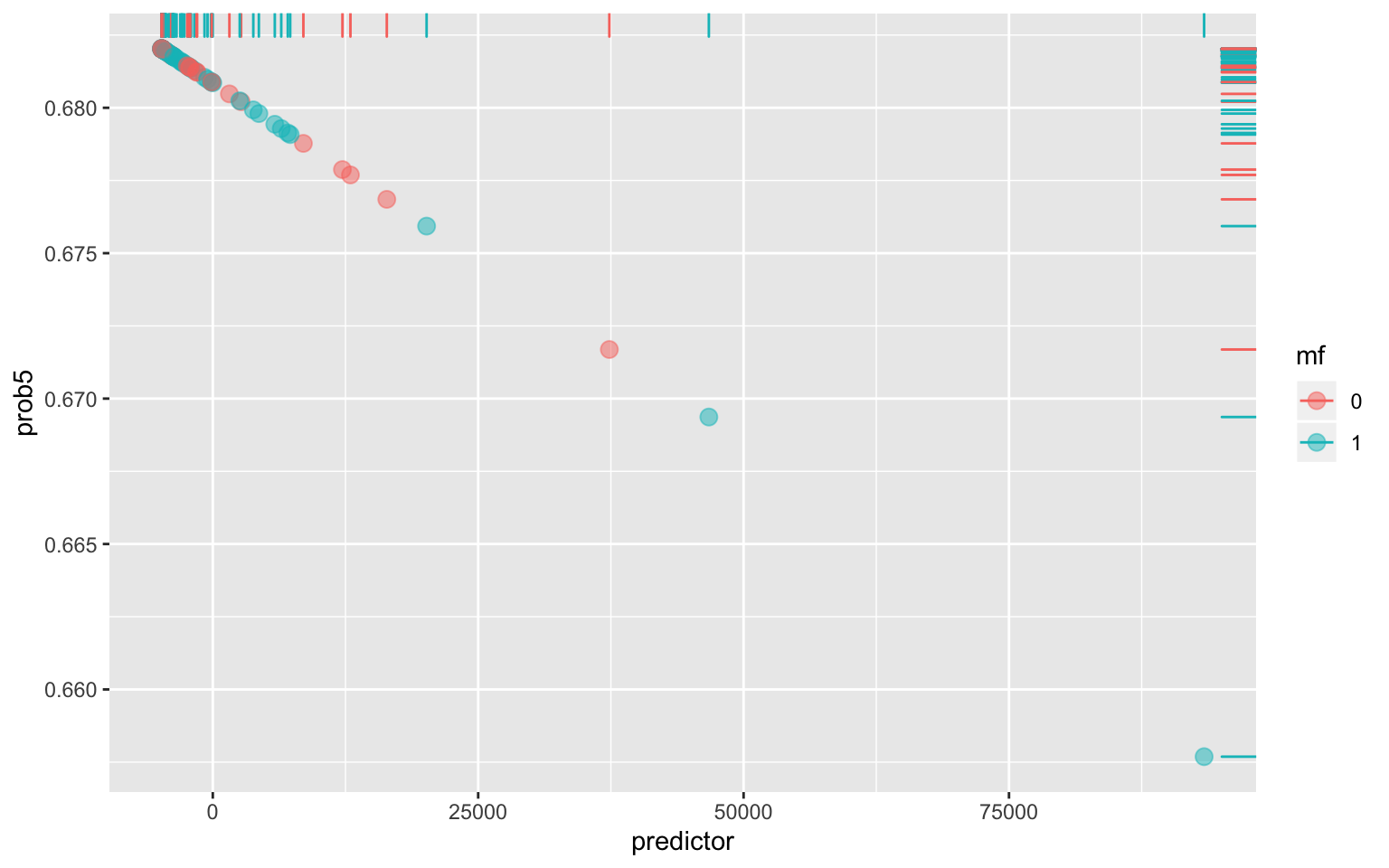

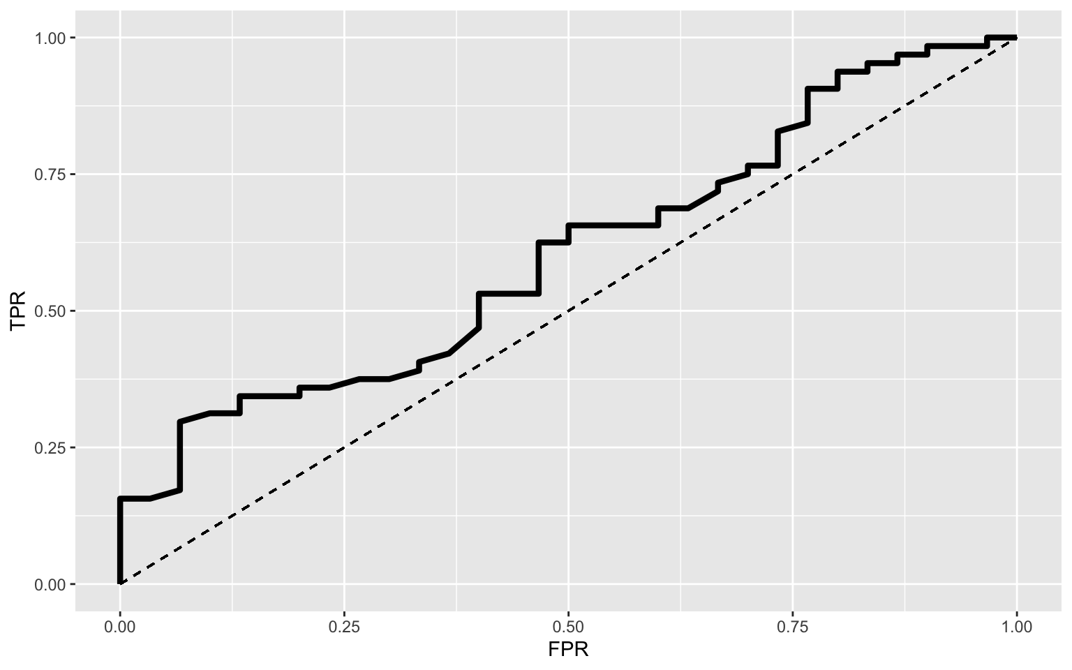
- Generating an ROC curve and calculating AUC

tpr <- function(p) mean(hurricane[hurricane$mf == 1, ]$prob > 
    p)
fpr <- function(p) mean(hurricane[hurricane$mf == 0, ]$prob > 
    p)
data <- hurricane[order(hurricane$prob), ]
prob <- hurricane$prob
cuts <- unique(c(0, (prob[-1] + prob[-32])/2, 1))
TPR <- sapply(cuts, tpr)
FPR <- sapply(cuts, fpr)
ROC1 <- data.frame(cuts, TPR, FPR, TP = TPR * 13, FP = FPR * 
    19) %>% arrange(desc(cuts))
ggplot(ROC1) + geom_path(aes(FPR, TPR), size = 1.5) + geom_segment(aes(x = 0, 
    y = 0, xend = 1, yend = 1), lty = 2) + scale_x_continuous(limits = c(0, 
    1))

widths <- diff(ROC1$FPR)
heights <- (ROC1$TPR[-1] + ROC1$TPR[-length(ROC1$TPR)])/2
AUC <- sum(heights * widths)
AUC

## [1] 0.603125

The AUC of this model is 0.603125 which is low. From the above ROC plot, the AUC is quite low, which means that this model is much closer to a “chance prediction” (AUC value of 0.5) as opposed to a “perfect prediction” (AUC value of 1.0). This can be interpreted as the probability that a randomly selected hurricane with a female name has about the same prediction as a randomly selected hurricane with a male name. These findings are quite anti-climactic as I was looking to find variation here, but it’s completely understandable as hurricanes are arbitrarily named far before they reach the US and cause severe damage. It would be silly to think the name has any effect on property damage levels or death levels, but I was looking at this for fun! (A small “what if…” went through my mind when performing this logistic regression and analysis)

- Performing a 10-fold Cross Validation (CV)

set.seed(1234)
k = 10
data1 <- hurricane[sample(nrow(hurricane)), ]
folds <- cut(seq(1:nrow(hurricane)), breaks = k, labels = F)
diags <- NULL
for (i in 1:k) {
    
    train <- data1[folds != i, ]
    test <- data1[folds == i, ]
    truth <- test$mf
    
    fit <- glm(mf ~ deaths + BaseDam2014, data = train, family = "binomial")
    probs <- predict(fit, newdata = test, type = "response")
    
    diags <- rbind(diags, class_diag(probs, truth))
}

apply(diags, 2, mean)

##       acc      sens      spec       ppv       auc 
## 0.6777778 0.9603175 0.1750000 0.6980952 0.5831429

For this 10-fold CV that was performed above, the average out-of-sample stats to report are: Accuracy = 0.68444444, Sensitivity = 0.97321429, and PPV (Recall) = 0.69250000.

• 6. Running a LASSO regression and inputting all the rest of the variables as predictors. Then, performing a 10-fold CV using this model.

hurricane6 <- hurricane %>% select(-c(Name, Year, damage_c, pressure_c, 
    wind_c, prob, Category, mf)) %>% na.omit()
hurricane6$LF.WindsMPH %>% as.numeric()

## [1] 120 130 85 85 85 120 120 145 120 85 120 105 145 120
85 120 145 85 145 85 105 105 120 105
## [25] 120 105 85 120 105 190 120 85 105 85 85 120 120 85
85 85 105 120 115 115 110 75 90 115
## [49] 120 85 100 85 75 75 80 80 140 85 105 170 115 100
115 105 115 80 110 80 105 115 105 80
## [73] 90 90 105 80 150 75 105 120 120 75 120 125 75 115
120 90 85 105 110 75 80 75

hurricane6$LF.PressureMB %>% as.numeric()

## [1] 958 955 985 987 985 960 954 938 962 987 960 975 945
946 984 950 930 981 931
## [20] 996 968 966 950 974 941 982 983 950 977 909 945 979
978 995 980 952 955 980
## [39] 995 986 970 946 945 962 949 1003 987 959 942 971
967 990 990 993 984 986 934
## [58] 983 962 922 961 973 942 974 954 984 964 987 964 951
956 987 963 979 957 972
## [77] 941 985 960 946 950 991 946 920 982 937 950 985 967
954 950 952 966 942

hurricane6$deaths %>% as.numeric()

## [1] 2 4 3 1 0 60 20 20 0 200 7 15 416 1 0 22 50 0 46
## [20] 3 3 5 37 3 75 6 3 15 3 256 22 2 0 0 117 1 21 5
## [39] 0 1 15 5 2 21 3 0 1 4 8 12 5 3 5 0 1 13 21
## [58] 3 15 62 3 6 9 8 26 10 3 3 1 0 56 8 2 3 51 1
## [77] 10 8 7 25 5 1 15 1836 1 62 5 1 1 52 84 41 5 159

y <- as.matrix(hurricane$NDAM2014)
x <- hurricane6 %>% dplyr::select(-NDAM2014) %>% mutate_all(scale) %>% 
    as.matrix
cv <- cv.glmnet(x, y)
lasso1 <- glmnet(x, y, lambda = cv$lambda.1se)

coef(lasso1)

## 7 x 1 sparse Matrix of class "dgCMatrix"
##                      s0
## (Intercept)   8433.0532
## LF.WindsMPH    575.7473
## LF.PressureMB -750.3565
## deaths           .     
## BaseDam2014   8209.7352
## predictor        .     
## prob5            .

set.seed(1234)
k = 10
data1 <- hurricane[sample(nrow(hurricane)), ]
folds <- cut(seq(1:nrow(hurricane)), breaks = k, labels = F)
diags <- NULL
for (i in 1:k) {
    
    train <- data1[folds != i, ]
    test <- data1[folds == i, ]
    truth <- test$NDAM2014
    
    fit <- lm(NDAM2014 ~ LF.WindsMPH + LF.PressureMB + BaseDam2014, 
        data = train)
    probs <- predict(fit, newdata = test, type = "response")
    
    diags <- rbind(diags, class_diag(probs, truth))
}

apply(diags, 2, mean)

##        acc       sens       spec        ppv        auc 
## 0.16111111 0.60000000 0.80000000 0.09007937 1.00000000

fit6 <- lm(NDAM2014 ~ LF.WindsMPH + LF.PressureMB + BaseDam2014, 
    data = train)
summary(fit6)

##
## Call:
## lm(formula = NDAM2014 ~ LF.WindsMPH + LF.PressureMB +
BaseDam2014,
## data = train)
##
## Residuals:
## Min 1Q Median 3Q Max
## -11311 -3877 -850 1195 46578
##
## Coefficients:
## Estimate Std. Error t value Pr(>|t|)
## (Intercept) -6.101e+04 9.211e+04 -0.662 0.509652
## LF.WindsMPH 2.444e+02 7.139e+01 3.423 0.000979 ***
## LF.PressureMB 4.098e+01 8.860e+01 0.463 0.644960
## BaseDam2014 9.419e-01 7.318e-02 12.870 < 2e-16 ***
## ---
## Signif. codes: 0 '***' 0.001 '**' 0.01 '*' 0.05 '.' 0.1
' ' 1
##
## Residual standard error: 7316 on 80 degrees of freedom
## Multiple R-squared: 0.8001, Adjusted R-squared: 0.7926
## F-statistic: 106.7 on 3 and 80 DF, p-value: < 2.2e-16

From running the LASSO regression, the variables that are retained are windspeeds (LF.WindsMPH), atmospheric pressure (LF.PressureMB), and the property damages (BaseDam2014). Unfortunately, because I used a numeric variable in the regression, I’m not sure how to compare RMSEs to find how well it ended up fitting.

…